library(tidyverse)
library(owidapi)
library(scales)
library(ggeasy)
library(janitor)
library(feathers)day 7 outliers
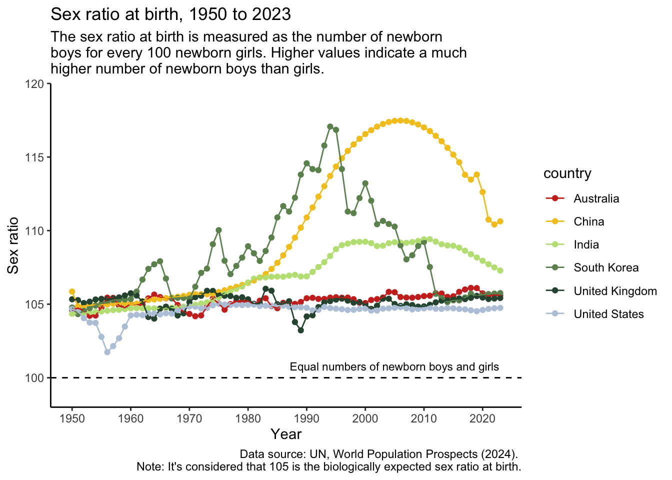
The plots at Our World in Data unpacking changes in sex ratio at birth across the world uncover some interesting outliers. Across the world it is typical for there to be slightly more boys born than girls. The sex ratio at conception is equal but across pregnancy, the risk of miscarriage is slightly higher for female than male fetuses, resulting in an average of 105 male to 100 female live births. But countries like China, India, and South Korea have much higher than average sex ratios.
I am going to reproduce this plot, adding the US, UK and Australia in for comparison.
load packages
read the data
Here I am reading in the data, cleaning names and renaming variables.
ratio <- read_csv("https://ourworldindata.org/grapher/sex-ratio-at-birth.csv?v=1&csvType=full&useColumnShortNames=true") %>%
  clean_names() %>%
  rename(country = entity, ratio = sex_ratio_sex_all_age_0_variant_estimates)
clean it up
I am filtering the data to include only China, India, and South Korea, as well as Australia, United States, and United Kingdom for comparison.
countries <- c("China", "India", "South Korea", "Australia", "United States", "United Kingdom")

ratio4 <- ratio %>%
  filter(country %in% countries)
plot
ratio4 %>%
  ggplot(aes(x = year, y = ratio, colour = country)) +
  geom_point() +
geom_line() 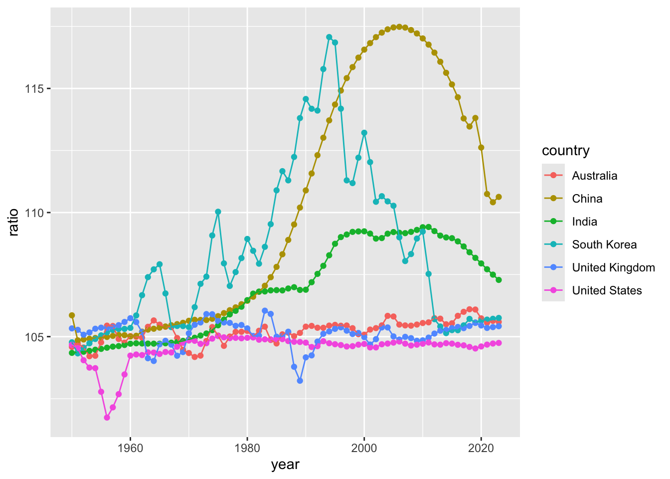
Basic plot check! Things I would like to change…
- background theme and axis labels
- horizontal line at 100
- colour palette
- titles and captions
theme, hline, and labels
ratio4 %>%
  ggplot(aes(x = year, y = ratio, colour = country)) +
  geom_point() +
  geom_line() +
  theme_classic() +
  scale_y_continuous(expand = c(0,0), limits = c(95, 120)) +
  scale_x_continuous(breaks = seq(1950, 2020, 10)) +
  geom_hline(yintercept = 100, linetype = 2) +
  geom_text(data = data.frame(x = 2005, y = 100.8, label = "Equal numbers of newborn boys and girls"), mapping = aes(x = x, y = y, label = label), size = 3, inherit.aes = FALSE) +
  labs(y = "Sex ratio", x = "Year")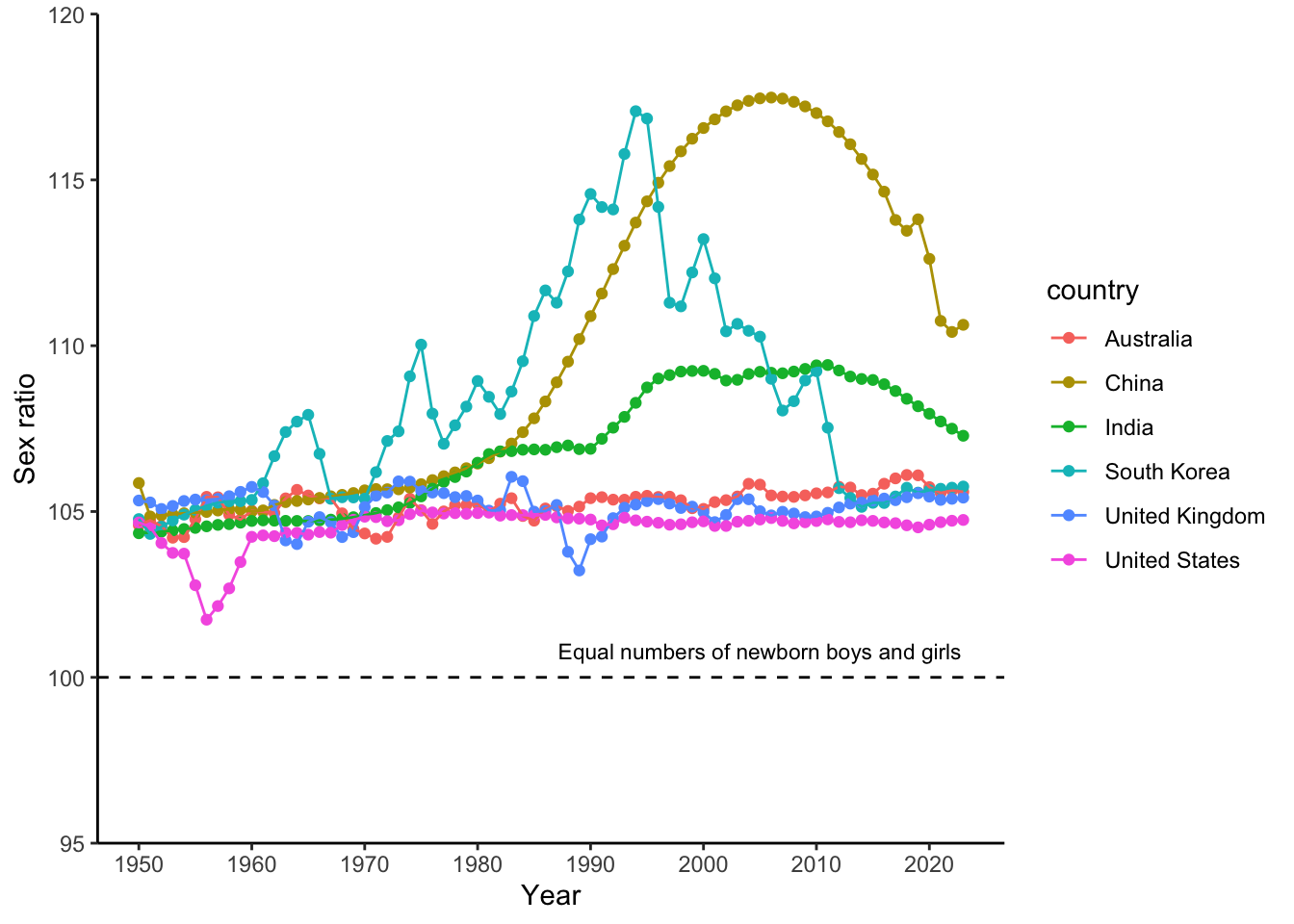
colours, titles, and captions
Practicing using a new palette package for this one; this time Aussie birds from the feathers package.
ratio4 %>%
  ggplot(aes(x = year, y = ratio, colour = country)) +
  geom_point() +
  geom_line() +
  theme_classic() +
scale_colour_manual(values = get_pal("eastern_rosella")) +
  scale_y_continuous(expand = c(0,0), limits = c(98, 120)) +
  scale_x_continuous(breaks = seq(1950, 2020, 10)) +
  geom_hline(yintercept = 100, linetype = 2) +
  geom_text(data = data.frame(x = 2005, y = 100.8, label = "Equal numbers of newborn boys and girls"), mapping = aes(x = x, y = y, label = label), size = 3, inherit.aes = FALSE) +
  labs(y = "Sex ratio", x = "Year",
       title = "Sex ratio at birth, 1950 to 2023",
       subtitle = "The sex ratio at birth is measured as the number of newborn \nboys for every 100 newborn girls. Higher values indicate a much \nhigher number of newborn boys than girls.",
       caption = "Data source: UN, World Population Prospects (2024). \nNote: It's considered that 105 is the biologically expected sex ratio at birth.")