library(tidyverse)
library(janitor)
library(ggeasy)
library(RColorBrewer)day 9_diverging
Our World in Data has a series of plots that report data from the Integrated Values survey, asking people across the world how important they consider a range of life areas (family, friends,work, leisure time, politics, religion. For the Day 6 prompt, I am wondering whether our views on the relative importance of family and work have shifted over time.
load packages
read/combine data
A bit of wrangling required for this one, because the data for each life area was in a different csv file. In this rather long code chunk, I am reading each csv in, cleaning up names, selecting relavant columns, adding a new column for life area, making the data long, and changing the string values in the ratings column to make them consistent (i.e. instead of very_important_in_life_family -> very_important_in_life).
Code
family <- read_csv("https://ourworldindata.org/grapher/how-important-family-is-to-people-in-life.csv?v=1&csvType=full&useColumnShortNames=true") %>%
  clean_names() %>%
  select(country = entity, year, ends_with("family")) %>%
  mutate(life_area = "family") %>%
  pivot_longer(names_to = "rating", values_to = "score", very_important_in_life_family:no_answer_important_in_life_family) %>%
  mutate(rating = str_sub(rating, 1, -8)) # edit string, start at pos1, end 8 chars back

friends <-  read_csv("https://ourworldindata.org/grapher/how-important-friends-are-to-people-in-life.csv?v=1&csvType=full&useColumnShortNames=true") %>%
  clean_names() %>%
  select(country = entity, year, ends_with("friends")) %>%
  mutate(life_area = "friends") %>%
  pivot_longer(names_to = "rating", values_to = "score", very_important_in_life_friends:no_answer_important_in_life_friends) %>%
  mutate(rating = str_sub(rating, 1, -9))

leisure <- read_csv("https://ourworldindata.org/grapher/how-important-leisure-is-to-people-in-life.csv?v=1&csvType=full&useColumnShortNames=true") %>%
  clean_names() %>%
  select(country = entity, year, ends_with("leisure_time")) %>%
  mutate(life_area = "leisure_time") %>%
  pivot_longer(names_to = "rating", values_to = "score", very_important_in_life_leisure_time:no_answer_important_in_life_leisure_time) %>%
  mutate(rating = str_sub(rating, 1, -14))

politics <- read_csv("https://ourworldindata.org/grapher/how-important-politics-is-in-your-life.csv?v=1&csvType=full&useColumnShortNames=true") %>%
  clean_names() %>%
  select(country = entity, year, ends_with("politics")) %>%
  mutate(life_area = "politics") %>%
  pivot_longer(names_to = "rating", values_to = "score", very_important_in_life_politics:no_answer_important_in_life_politics) %>%
  mutate(rating = str_sub(rating, 1, -10))

religion <-read_csv("https://ourworldindata.org/grapher/how-important-religion-is-in-your-life.csv?v=1&csvType=full&useColumnShortNames=true") %>%
  clean_names() %>%
  select(country = entity, year, ends_with("religion")) %>%
  mutate(life_area = "religion") %>%
  pivot_longer(names_to = "rating", values_to = "score", very_important_in_life_religion:no_answer_important_in_life_religion) %>%
  mutate(rating = str_sub(rating, 1, -10))

work <- read_csv("https://ourworldindata.org/grapher/how-important-work-is-to-people-in-life.csv?v=1&csvType=full&useColumnShortNames=true") %>%
  clean_names() %>%
  select(country = entity, year, ends_with("work")) %>%
  mutate(life_area = "work") %>%
  pivot_longer(names_to = "rating", values_to = "score", very_important_in_life_work:no_answer_important_in_life_work) %>%
  mutate(rating = str_sub(rating, 1, -6))
Once I have separate dataframes for each life area that are all structured in the same way, I can use rbind() to join them all togeher.
life <- rbind(family, friends, leisure, work, politics, religion)clean it up
A little more string editing, this time chopping the _in_life piece of the end of each of the rating strings and converting both rating and life area to factors.
life_ratings <- life %>%
  mutate(rating = str_sub(rating, 1, -9)) %>%
  mutate(rating = as_factor(rating)) %>%
  mutate(life_area = as_factor(life_area))

glimpse(life_ratings)
Rows: 14,328
Columns: 5
$ country <chr> "Albania", "Albania", "Albania", "Albania", "Albania", "Alba…
$ year <dbl> 1998, 1998, 1998, 1998, 1998, 1998, 2004, 2004, 2004, 2004, …
$ life_area <fct> family, family, family, family, family, family, family, fami…
$ rating <fct> very_important, rather_important, not_very_important, notata…
$ score <dbl> 95.7958000, 3.2032030, 0.3003003, 0.2002002, 0.5005005, 0.00…I am using the same selection of countries that I plotted in my sex ratio chart, for no good reason really. I am interested in just data for the family and work life areas and want to sum the proportion of people that have “very important” and “rather important” ratings so group the data by year, country and life area and sum the scores.
countries <- c("China", "India", "South Korea", "Australia", "United States", "United Kingdom")
f_w <- c("family", "work")
impt <- c("very_important", "rather_important")

work_family <- life_ratings %>%
  filter(life_area %in% f_w) %>%
  filter(country %in% countries) %>%
  filter(rating  %in% impt) %>%
  group_by(year, country, life_area) %>%
  summarise(important = sum(score)) %>%
  ungroup()
`summarise()` has grouped output by 'year', 'country'. You can override using
the `.groups` argument.plot family and work
work_family %>%
  ggplot(aes(x = year, y = important, colour = life_area)) +
  geom_point() +
  geom_line() +
  facet_wrap(~ country) +
  labs(title = "Percent of people who rate family and work as `very important` \nor `rather important`")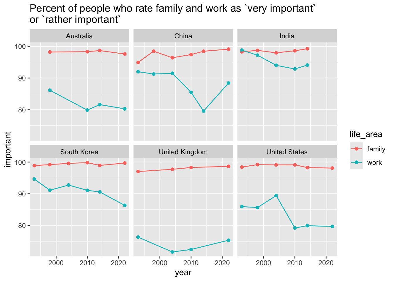
Basic plot check! Things I would like to change…
- theme and axis labels
- scale issues
- colour scheme
- add subtitle caption
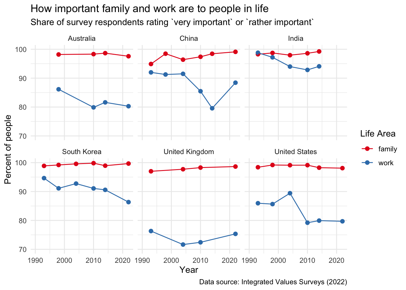
work_family %>%
  ggplot(aes(x = year, y = important, colour = life_area)) +
  geom_point(size = 2) +
  geom_line() +
  facet_wrap(~ country) +
  labs(title = "How important family and work are to people in life",
       subtitle = "Share of survey respondents rating `very important` or `rather important`",
       x = "Year", y = "Percent of people",
       caption = "Data source: Integrated Values Surveys (2022)") +
  theme_minimal() +
  scale_y_continuous(limits = c(70,100)) +
  scale_x_continuous(limits = c(1990, 2022)) +
  scale_color_brewer(palette = "Set1") +
  easy_add_legend_title("Life Area")