library(tidyverse)library(tidytuesdayR)library(tidyplots)library(janitor)library(ggpubr)library(here)# choosing a dataset randomlyset.seed(4)ttyears <-c(2018:2025)ttweeks <-c(1:52)# choose a year at randomchosen_year <-sample(ttyears, size =1)# choose at week at randomchosen_week <-sample(ttweeks, size =1)# read the data from that year/weekdf <- tidytuesdayR::tt_load(chosen_year, chosen_week)# print datasetprint(df)palm <- df[[1]]options(scipen =999)
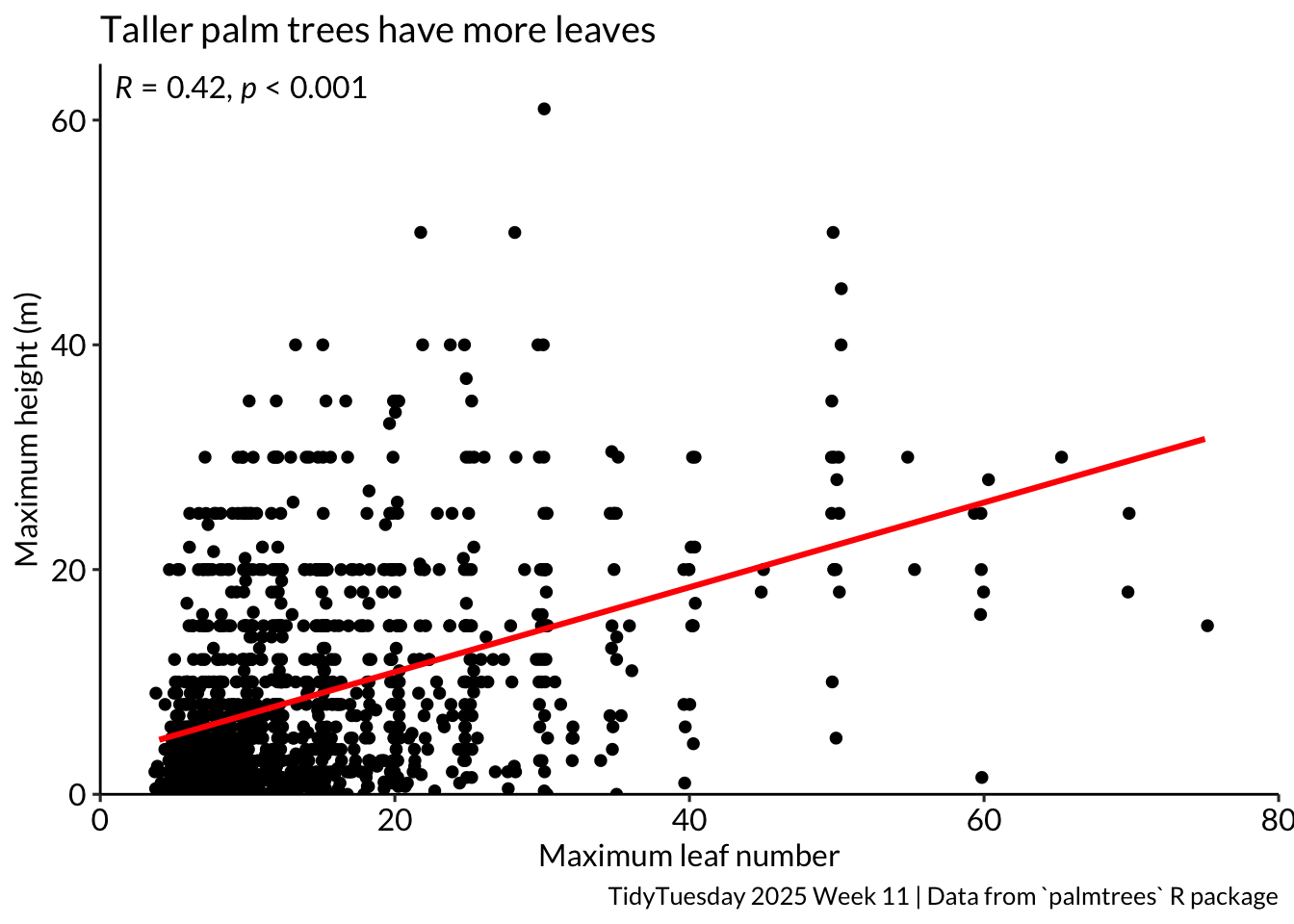
The data for this plot comes from a 2025 TidyTuesday challenge. The Week 11 data that year was about Palm Trees.
ggplot
Code
palm |>ggplot(aes(y = max_stem_height_m, x = max_leaf_number)) +geom_jitter() +scale_y_continuous(limits =c(0,65), breaks =seq(0,80,20), expand =c(0,0)) +scale_x_continuous(limits =c(0,80), breaks =seq(0,80,20), expand =c(0,0)) +geom_smooth(method ="lm", se =FALSE, colour ="red") +labs(y ="Maximum height (m)", x ="Maximum leaf number", title ="Taller palm trees have more leaves", caption ="TidyTuesday 2025 Week 11 | Data from `palmtrees` R package") +theme_pubr(base_family ="Lato") +stat_cor(method ="pearson", p.accuracy =0.001, r.accuracy =0.01, label.x =1)
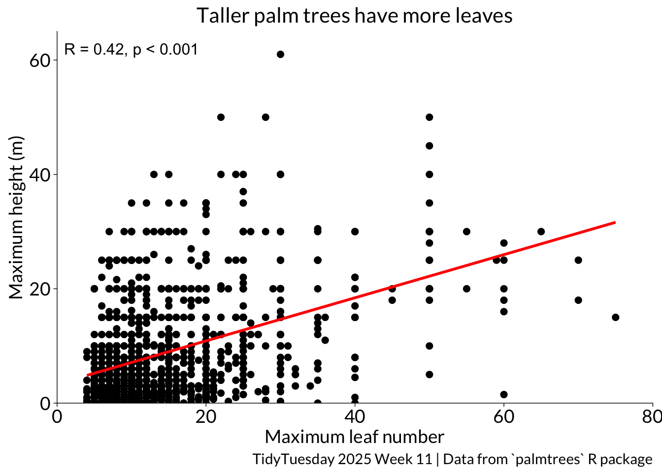
tidyplot
Code
palm |>tidyplot(y = max_stem_height_m, x = max_leaf_number) |>add_data_points_jitter(colour ="black", size =2) |>add_curve_fit(method ="lm", colour ="red", linewidth =1, se =FALSE) |>adjust_y_axis(limits =c(0,65), breaks =seq(0,80,20)) |>adjust_x_axis(limits =c(0,80), breaks =seq(0,80,20)) |>adjust_font(fontsize =14, family ="Lato") |>adjust_title("Taller palm trees have more leaves", fontsize =16) |>adjust_x_axis_title("Maximum leaf number") |>adjust_y_axis_title("Maximum height (m)") |>adjust_caption("TidyTuesday 2025 Week 11 | Data from `palmtrees` R package") |>adjust_size(unit ="mm", width =160, height =100) |>add_annotation_text("R = 0.42, p < 0.001", x =10, y =62, fontsize =12) |>save_plot(here::here("charts26", "2026-04-04_slope","tidyfeatured.png"))