day 11: physical

library(tidyverse)
library(tidytuesdayR)
library(tidyplots)
library(janitor)
library(ggeasy)
library(here)
library(RColorBrewer)


# read the data from that year/week

chosen_year <- 2026
chosen_week <- 13

df <- tidytuesdayR::tt_load(2026, 13)



# print dataset
print(df)

temp <- df[[1]]


options(scipen = 999)

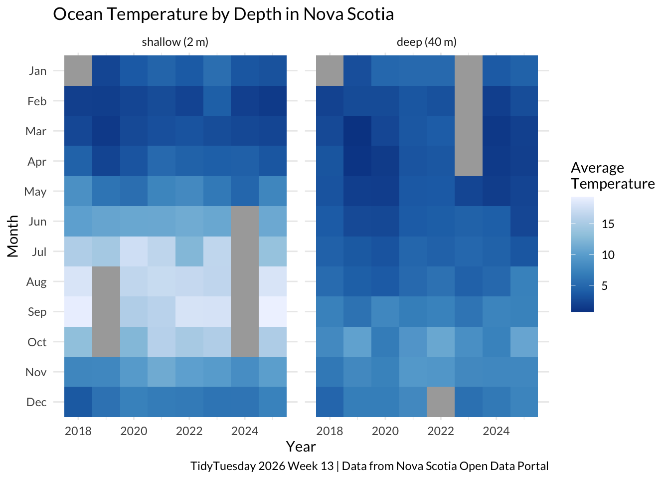
The data for this plot comes from a 2026 TidyTuesday challenge. The Week 13 data that year was about ocean temperature in Nova Scotia.

prep

shallow_deep <- temp %>%
  filter(sensor_depth_at_low_tide_m %in% c(2, 40)) %>%
  group_by(sensor_depth_at_low_tide_m, year(date), month(date)) %>%
  summarise(monthly_mean = mean(mean_temperature_degree_c)) %>%
  rename(month = "month(date)", year = "year(date)", depth = sensor_depth_at_low_tide_m) %>%
  mutate(depth = case_when(depth == 2 ~ "shallow (2 m)", 
                           depth == 40 ~ "deep (40 m)")) %>%
  mutate(depth = as.factor(depth)) %>%
  mutate(depth = fct_relevel(depth, c("shallow (2 m)", "deep (40 m)"))) %>%
  mutate(month = factor(month, levels = 1:12, labels = month.abb)) %>%
  arrange(depth, year, month) %>%
  ungroup() 


# make missing data explicit NA

shallow_deep_complete <- shallow_deep %>%
  complete(year, month = factor(month, levels = month.abb), depth) %>%
   mutate(month = forcats::fct_rev(month))

ggplot

shallow_deep_complete %>%
  ggplot(aes(x = year, y = month, fill = monthly_mean)) +
  geom_tile() +
  facet_wrap(~depth) +
  theme_minimal(base_family = "Lato") +
  scale_fill_distiller(palette = "Blues", na.value = "darkgrey",
                      name = "Average \nTemperature") +
  labs(y = "Month", x = "Year", title = "Ocean Temperature by Depth in Nova Scotia", 
       caption = "TidyTuesday 2026 Week 13 | Data from Nova Scotia Open Data Portal") 

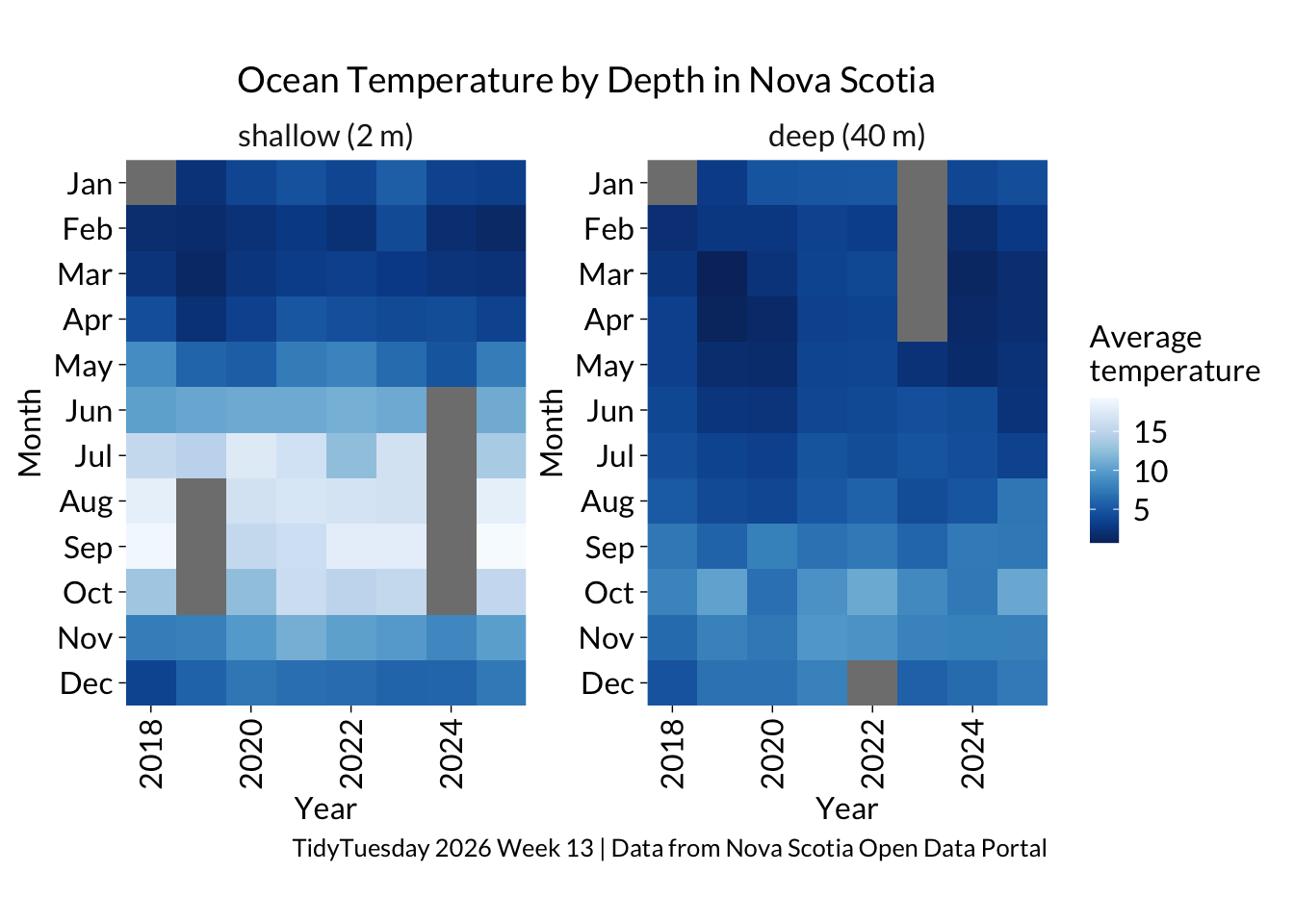
tidyplot

blues <- brewer.pal(9, "Blues")


shallow_deep_complete %>%
  tidyplot(x = year, y = month, fill = monthly_mean) %>%
  add_heatmap() %>%
  split_plot(by = depth) %>%
   adjust_size(width = 55, height = 75) %>%
  adjust_font(fontsize = 12, family = "Lato") %>%
  adjust_title("Ocean Temperature by Depth in Nova Scotia", fontsize = 14) %>%
  adjust_colors(new_colors = rev(blues)) %>%
  adjust_caption("TidyTuesday 2026 Week 13 | Data from Nova Scotia Open Data Portal") %>%
  adjust_x_axis_title("Year") %>%
  adjust_y_axis_title("Month") %>%
  adjust_legend_title("Average \ntemperature") %>%
  save_plot(here::here("charts26", "2026-04-11_physical", "tidyfeatured.png"))