Day 7: accessibility

I am interested in the accessibility of public libraries.

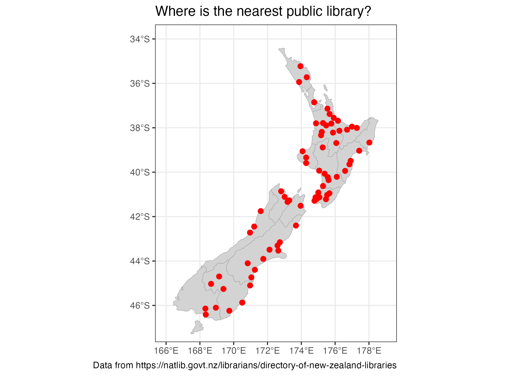
Here I worked out how to plot library locations on a map that also included regional information. The map below does make me question how complete the Directory of New Zealand libraries is though. Surely there is more than 1 library in Auckland!

load packages

library(tidyverse)
library(here)
library(janitor)
library(tidygeocoder)
library(spData)
library(sf)

get data

The geocode() function is amazing at turning address data into lat/long data but SLOW when it is looking for more than a handful of coordinates, so here I am writing the data to csv in order to read it back in.

Tried method = “osm” first (OpenStreetMap) and it missed coordinates for 23 sites. Turns out that method = “arcgis” works better.

cities <- c("Auckland", "Hamilton", "Wellington", "Christchurch", "Dunedin")

libraries <- read_csv("maps/2025-11-07_accessibility/directory-of-new-zealand-libraries.csv") %>%
  clean_names() %>%
   mutate(city = str_extract(street_address, paste(cities, collapse = "|"))) %>%
select(library_type_3, name, street_address, city) 


public <- libraries %>%
  filter(library_type_3 == "Public") %>%
  geocode(street_address, method = 'arcgis', lat = latitude , long = longitude) 


public %>% 
  filter(library_type_3 == "Public") %>%
  write_csv(here("maps", "2025-11-07_accessibility", "public.csv"))

plot1

If you want to make a map without regional information using the rnaturalearth package works well.

lib <- read_csv(here("maps", "2025-11-07_accessibility", "public.csv")) 

rne_nz <- rnaturalearth::ne_countries(country = "new zealand", returnclass = "sf", scale = "large")


ggplot() +
  geom_sf(data = rne_nz) +
  geom_point(data = lib, aes(x = longitude, y = latitude)) +
  coord_sf(xlim = c(166, 179), ylim = c(-47, -34)) +
  theme_bw()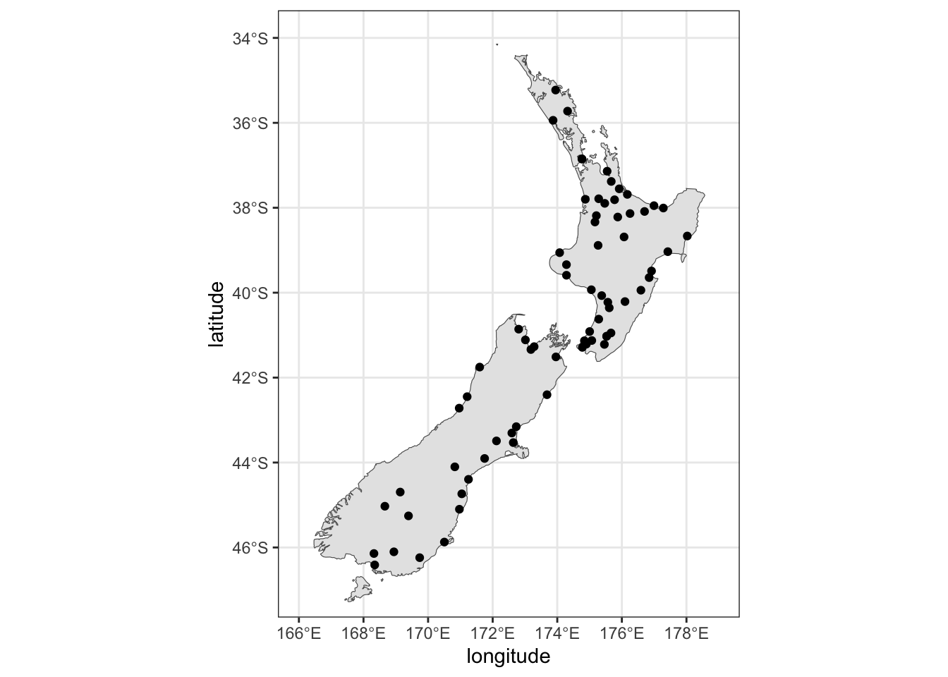

plot2

But if you want regional information on your plot, you need to battle wih spData. Here I ran into problems that required converting the nz map to lat/long and then converting point locations to sf.

# nz map with areas from spData 

nz <- nz

sp_nz <- st_transform(nz, 4326)  # Convert nz to lat/long

# convert points to sf geometry

lib_sf <- st_as_sf(lib, coords = c("longitude", "latitude"), crs = 4326)

ggplot() +
  geom_sf(data = sp_nz, fill = "lightgrey", color = "darkgrey") +
  geom_sf(data = lib_sf, color = "red", size = 2) +
  coord_sf(xlim = c(166, 179), ylim = c(-47, -34)) +
  theme_bw() +
  labs(title = "Where is the nearest public library?", caption= "Data from https://natlib.govt.nz/librarians/directory-of-new-zealand-libraries")