gas prices

tidy tuesday week 26

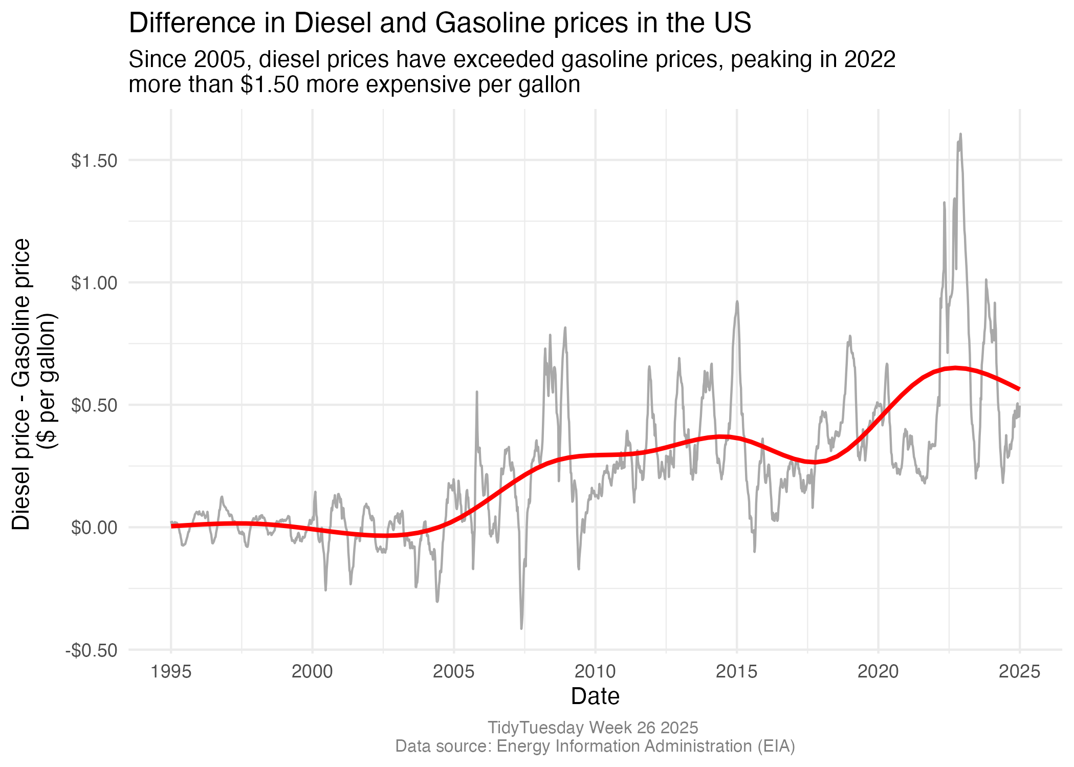
The TidyTuesday data this week are about gasoline and diesel prices in the US. I have plotted the price differential between regular gasoline and diesel.

get data

library(tidyverse)
library(tidytuesdayR)
library(Hmisc)
library(scales)

tt <-  tt_load(2025, week = 26)

gas <- tt$weekly_gas_prices

wrangle

I want to get the difference between diesel and gasoline prices and my first instinct is to make the data wide and when subtract across columns. Here I worked out how to get difference scores without making the data wide first.

group_by |> mutate

g_long <- gas %>%
  filter(
    fuel == "diesel" & grade == "all" |
    (fuel == "gasoline" & grade == "regular" & formulation == "all")) %>%
  select(date, fuel, price) %>%
  filter(date >= "1994-03-21") %>%
  group_by(date) %>%
  mutate(diff = price[fuel == "diesel"] - price[fuel == "gasoline"]) %>%
  ungroup()

pivot_wider |> rowwise |> mutate

g_wide <- gas %>%
  filter(
    fuel == "diesel" & grade == "all" |
    (fuel == "gasoline" & grade == "regular" & formulation == "all")) %>%
  select(date, fuel, price) %>%
  filter(date >= "1994-03-21") %>%
  pivot_wider(names_from = fuel, values_from = price) %>%
  rowwise() %>%
  mutate(diff = diesel - gasoline) %>%
  ungroup()

plot

g_long %>%
  filter(fuel == "gasoline") %>%
  ggplot(aes(x = date, y = diff)) +
  geom_line(colour = "darkgrey") +
  geom_smooth(se = FALSE, colour = "red") +
  labs(y = "Diesel price - Gasoline price \n($ per gallon)", x = "Date", 
       title = "Difference in Diesel and Gasoline prices in the US", 
       subtitle = "Since 2005, diesel prices have exceeded gasoline prices, peaking in 2022 \nmore than $1.50 more expensive per gallon", 
       caption = "TidyTuesday Week 26 2025 \nData source: Energy Information Administration (EIA)") +
  scale_x_date(
        breaks = seq(as.Date("1995-01-01"), as.Date("2025-01-01"), by = "5 years"),
        date_labels = "%Y",
        limits = c(as.Date("1995-01-01"), as.Date("2025-01-01"))) +
  scale_y_continuous(labels = dollar_format()) +
  theme_minimal()  +
  theme(plot.caption = element_text(hjust = 0.5, size = 8, color = "gray50"))