Code
library(tidyverse)
library(janitor)
library(ggeasy)
library(tidytuesdayR)
library(sf)
library(plotly)
library(htmlwidgets)


year = 2025
week = 33

tt <- tt_load(year, week)

munros <- tt[[1]] %>%
clean_names() TidyTuesday Week 33
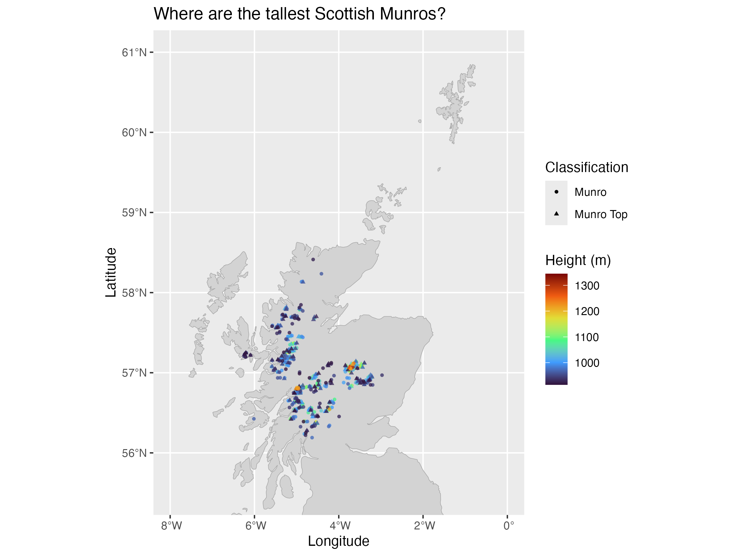
Trying my hand at a map for Tidy Tuesday this week. This plot illustrates the location and elevation of Scottish Munros. The plotly package makes it super easy to take a ggplot and make it interactive.
library(tidyverse)
library(janitor)
library(ggeasy)
library(tidytuesdayR)
library(sf)
library(plotly)
library(htmlwidgets)
year = 2025
week = 33
tt <- tt_load(year, week)
munros <- tt[[1]] %>%
clean_names() munros_map <- munros %>%
select(do_bih_number, name, xcoord, ycoord, height_m, Classification = x2021) %>%
na.omit()
# Convert OSGB36 coordinates to sf object
munros_sf <- munros_map %>%
st_as_sf(coords = c("xcoord", "ycoord"),
crs = 27700) # EPSG:27700 is OSGB36 / British National Grid
# Transform to WGS84 (lat/long) for easier plotting
munros_lat_long <- munros_sf %>%
st_transform(crs = 4326)
# Extract coordinates for ggplot
munros_coords <- munros_lat_long %>%
mutate(
longitude = st_coordinates(.)[,1],
latitude = st_coordinates(.)[,2]
) %>%
st_drop_geometry() %>%
arrange(-height_m)uk_map <- rnaturalearth::ne_countries(scale = "large",
country = "United Kingdom",
returnclass = "sf")
plot <- ggplot() +
geom_sf(data = uk_map, fill = "lightgray", color = "darkgrey", size = 0.3) +
geom_point(data = filter(munros_coords, height_m < 1200), aes(x = longitude, y = latitude, shape = Classification, label = name, colour = height_m), size = 1, alpha = 0.8) +
geom_point(data = filter(munros_coords, height_m >= 1200), aes(x = longitude, y = latitude, shape = Classification, label = name, colour = height_m), size = 1, alpha = 0.8) +
scale_color_viridis_c(name = "Height (m)",
option = "turbo") +
coord_sf(xlim = c(-8, 0), ylim = c(55.5, 61)) +
labs(y = "Latitude", x = "Longitude", title = "Where are the tallest Scottish Munros?") +
theme_bw()
ggsave(here::here("tidytuesday", "2025-08-19_munros", "featured.png"), width = 8, height = 6, bg = "white")